【数据可视化】世界杯冠军预测
汪雨晨 数据智农
世界杯冠军预测代码
一、导入库
import pandas as pd
import numpy as np
import os
import matplotlib.pyplot as plt
import seaborn as sns
from wordcloud import WordCloud
二、读取数据
#read Data
world_cups=pd.read_csv("C:\\kaggle\\world\\WorldCups.csv")
world_cup_players=pd.read_csv("C:\\kaggle\\world\\WorldCupPlayers.csv")
world_cup_matches=pd.read_csv("C:\\kaggle\\world\\WorldCupMatches.csv")
三、计算不同国家队伍获得冠军次数
(1)程序:
fig=plt.figure()
winner=world_cups[Winner].value_counts()
winner.plot(kind=bar,title="Champion of FIFA World Cup",fontsize=14,figsize=(12,10))
plt.xlabel(Teams)
plt.ylabel(Number of Winnings)
plt.show()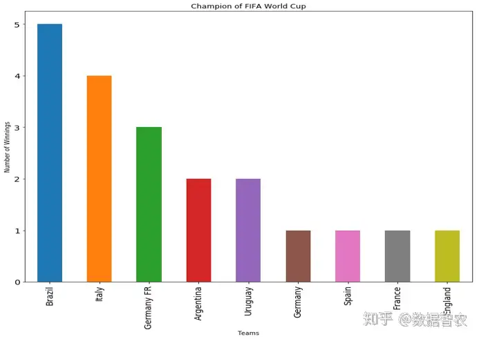
(2)分析结果:
从条形图结果可以直观的看出,获得世界杯冠军次数最多的三个国家分别是巴西、意大利和西德国,阿根廷以及乌拉圭获得世界杯冠军的次数与前三个国家相比次数较少。图中获得世界杯冠军次数最少的国家是德国(1990年后东西德国合体)、西班牙、法国、英格兰,都只有过一次夺冠经历。
四、统计历年世界杯参与人数
(1)程序:
#attendance of crowd in WorldCup from 1930 to 2014
world_cups[Attendance]=world_cups[Attendance].apply(lambda x:x.replace(.,))#删除小数点
Crowd=world_cups[[Year,Attendance]]
Crowd
plt.figure(figsize=(15,8))
sns.barplot(Crowd[Year].astype(int),Crowd[Attendance].astype(int))
plt.ylabel(Attendance)
plt.xlabel(Year)
plt.title(Crowd present at stadium in year 1930 to 2014)
plt.show()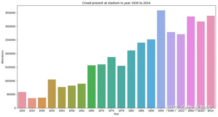
(2)分析结果:
从上图结果可以看出随着时间的变化参加世界杯比赛的人数在增加,虽然数据出现了一些波动,但整体呈上升趋势,可见越来越多人愿意投入到世界杯比赛及足球运动当中。
五、统计历年世界杯进球次数
(1)程序:
goal=world_cups[[Year,GoalsScored]]
plt.figure(figsize=(16,8))
plt.plot(goal[Year],goal[GoalsScored],-p,color=gray,markersize=15,linewidth=6,markerfacecolor=white,markeredgecolor=gray)
plt.xlim(1930,2018)
plt.ylim(60,180)
plt.xlabel(Year,fontstyle=italic)
plt.ylabel(GoalScored)
plt.show()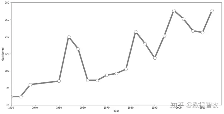
(2)分析结果
折线图直观地展示了历年的进球数量,其中1950年-1954年进球数量增幅最大,1954年-1960年也体现出了强烈的下降趋势,但整体图像并没有体现出一定的趋势,也没有体现出一定的规律性,如果想要的最后的预测结果还需进行其他操作。
六、计算每一场比赛参与人数
(1)程序:
#Average attendance of the crowd in WorldCup Matches from 1930 to 2014
#avg_att=np.array(world_cups[Attendance].astype(int))/np.array(world_cups[MatchesPlayed].astype(int))
#avg_att=np.transpose(avg_att)
#avg_att1=world_cups.groupby(world_cups[Year],avg_att)
avg_att = world_cup_matches.groupby(Year)[Attendance].mean().reset_index()
#按照‘Year’进行分组计算Attendance的均值
# 可以理解为avg_att=world_cups[Attendance]/world_cups[MatchesPlayed]每一场比赛参与人数
plt.figure(figsize=(15,8))
plt.plot(avg_att[Year],avg_att[Attendance],-p,linewidth=4,color=gray,markersize=12)
plt.xlabel(Year)
plt.ylabel(Attendance)
plt.title(Average attendance of crowd in WorldCup Matches)
plt.grid(True)
plt.show()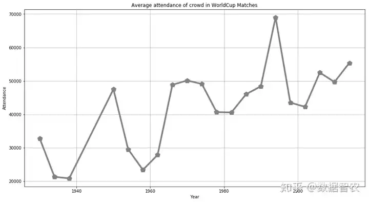
(2)分析结果
由于每次参加世界杯的球员并不能全部上场比赛,因此制作了每场比赛参与的人数折线图。折线图直观地展示了每一场比赛参与人数,其中1986年参与的人数最多,近几年参与比赛的人数也出现了缓慢的增长。同样,整体图像并没有体现出一定的趋势,也没有体现出一定的规律性,如果想要的最后的预测结果还需进行其他操作。
七、主队客队半场分数比较
7.1(1)程序
#Half time Goals of home and away team
Half_time=world_cup_matches.groupby(Year)[Half-time Home Goals,Half-time Away Goals].sum().reset_index().astype(int)
df=pd.DataFrame({Half-time Away Goals:Half_time[Half-time Away Goals],Half-time Home Goals:Half_time[Half-time Home Goals]})
df.plot(kind=bar,stacked=True,figsize=(18,15))
plt.title(Half time goals of home and away team)
r=range(0,20)
plt.xticks(r,Half_time[Year])
plt.xlabel(Year)
plt.show()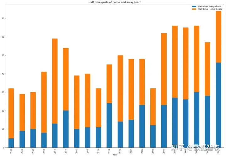
(2)分析结果
通过用两种不同的颜色对主客场球队的得分情况进行分析,结果显示,从整体趋势来看主场球队的半场得分具有压倒性优势,除了1974年及1986年两年出现了比分的差异性,从近几年的情况上看客场得分在逐渐上升,主客场的半场竞争力在不断减小。
7.2(1)程序
#主队
home_team1=world_cup_matches[[Year,Home Team Goals]]
home_team1.head(840)
home_team=world_cup_matches[[Year,Home Team Goals]].head(840).astype(int)
plt.figure(figsize=(15,10))
sns.violinplot(x=home_team[Year],y=home_team[Home Team Goals],palette=Blues)
plt.grid(True,color=grey,alpha=0.3)
plt.title("Home Team Goals")
plt.show()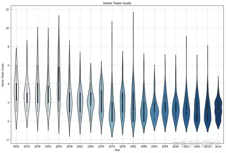
(2)分析结果:
通过对主队和客队分别进行分析,作图。首先可以通过以上小提琴图观察历年主队进球数的变化,从1930年-1954年间的图像可以看出,数值在3附近时密度最大,说明在这个时间段内大多数球队进球数为3个球。1958年-1970年这个时间段内数值在2附近密度最大,多数球队进球数为2个。从1970年-2014年,数值密度则稳定在1-3这个区域,每个球队的进球数也在1-3这个区间最多。
7.3(1)程序:
#客队 Away Team Goals
away_team=world_cup_matches[[Year,Away Team Goals]].head(840).astype(int)
plt.figure(figsize=(15,10))
sns.violinplot(x=away_team[Year],y=away_team[Away Team Goals],palette=Blues)
plt.grid(True,color=grey,alpha=0.3)
plt.title("Away Team Goals")
plt.show()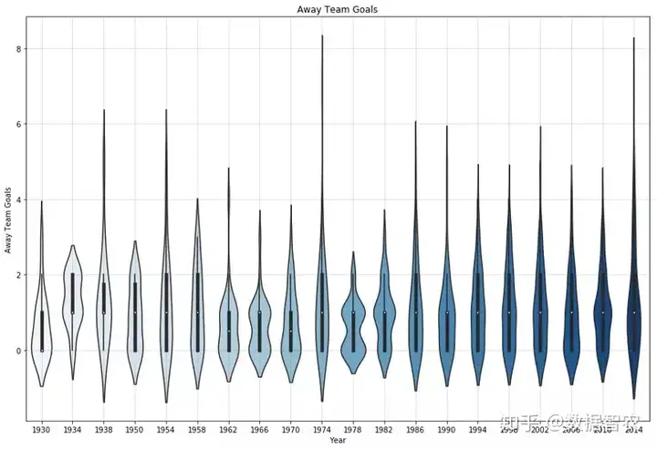
(2)分析结果:
客队得分数据在1930年-1982年这个区间波动较大,但最大密度分布区域在数值1-2附近,证明多数球队进球数为1-2个。然而1986年-2014年这个区间图像体现出了相似性,尤其在2014年,峰值在8附近,但密度很低,由于2014年世界杯出现了巴西对战德国1:7的大比分,这一事实也体现了图像和数据集的真实性和可操作性。
八、历年优秀球员统计
(1)程序:
#player names
from PIL import Image
plt.figure(figsize=(15,10))
name=np.array(Image.open(C:\\kaggle\\world\\7.png))
worldcloud=WordCloud(mask=name,max_words=5000).generate( .join(world_cup_players[Player Name]))
plt.imshow(worldcloud,interpolation=bilinear)
plt.axis(off)
plt.show()
(2)分析结果:
根据数据及给出的数据对历年参赛球员进行了词云分析,综合了参赛次数和得分情况绘制图像得出以上结果,可以看出,carlo所占比例最大也最为突出,Carlo是一名意大利球员,这一结果与之前的各国所得世界杯冠军次数结果也有一定的相关性,意大利确实在夺冠次数中表现优异。
九、世界杯冠军预测
(1)程序:
plt.figure(figsize=(15,10))
wordcloud=WordCloud( ).generate( .join(world_cup_matches[Home Team Name].head(840)))
plt.imshow(wordcloud,interpolation=bilinear)
plt.axis(off)
plt.show()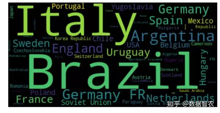
(3)分析结果:
综合上述分析,并结合了各国进球次数、参赛次数、得分情况绘制云图,对下一届世界杯夺冠球队进行预测分析。从上图可以看出,巴西、意大利、阿根廷、德国、英格兰占比较大,词汇也比较突出,其中巴西和意大利更加体现出了优势,可见巴西、意大利、阿根廷依然是下一届世界杯夺冠的热门球队。长按二维码关注
如有任何问题
您可以发送邮件至
dataintellagr@126.com
或关注微博/知乎/微信后台留言
我们期待您的提问!
微博:数据智农
知乎:数据智农
邮箱:dataintellagr@126.com
制作:孟子煜推荐阅读
-

梅西失点,阿根廷队2-0波兰,头名晋级16强,1/8决赛对阵澳大利亚(梅西阿根廷世界杯最好成绩)
-
阿根廷2-0波兰晋级16强 淘汰赛遇澳大利亚或取胜 阿根廷有望夺冠(波利维亚对阿根廷)
-

世界杯最新战报:个人第999场比赛罚失点球,梅西:我很生气!法国爆冷输给突尼斯,16强对阵:阿根廷VS澳大利亚,法国VS波兰(梅西世界杯射失点球技术确实不如内马尔)
-

11/16 中国 VS 澳大利亚 阿曼 VS 日本 阿根廷 VS 巴西(阿根廷vs日本男篮比分预测)
-

法国2-1险胜澳洲格子点射博格巴绝杀,阿根廷1-1冰岛梅西失点(中国胜法国平德国)
-

12/01周四世界杯二串分析:加拿大VS摩洛哥+克罗地亚VS比利时【16强赛事前夕】
-

加拿大vs摩洛哥赛前预测,周四世界杯串关分享
-
世界杯:加拿大vs摩洛哥,已经出局能否最后出力拼搏!比分预测!